What are Network Materials?

Network materials form a broad class encompassing engineering and biological materials. They have a network of filaments as their main structural element and the behavior of the network defines the macroscopic behavior of the material.

Most biomaterials are fibrous. This is due to several advantages offered by building with fibers: lightweight (with a small volume of material one can span large embedding volumes), adjustable stiffness obtained by anisotropic/preferential fiber orientations, large deformations without loss of carrying capacity.

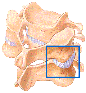
Connective tissue is made from collagen (and elastin) fibers, various membranes in the body, such as the liver capsule, basal membrane and the amnion are collagen networks, while each cell of our bodies has an internal network structure of fibrilar actin, the cytoskeleton, which embeds the cellular organelle and regulates cellular mechanics and mediates transport across the cytoplasm.

Network materials of the engineering world include molecular networks, such as rubber, epoxy and many other types of thermosets, and networks of fibers, such as textiles, nonwovens, paper and cellulose products, carbon nanotube buckypaper, etc.

Mechanical Behavior of Crosslinked Network Materials

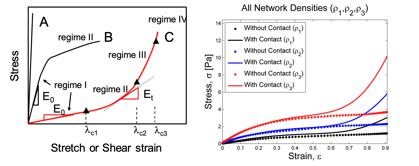
Based on their mechanical behavior, network materials can be divided in three classes – see Fig. 3. Materials from class A are brittle and have an approximately linear stress-strain curve up to or close to failure. Materials of class B have a concave stress-strain curve, with a yield-point which typically separates the elastic and plastic regions of the curve. Materials of class C are hyperelastic, stiffen continuously as they are stretched and follow the loading path during unloading (some degree of hysteresis is possible).

In compression, some network materials exhibit softening, followed by stiffening at large strains, as shown in Fig. 3. Other network materials which are embedded in a volume preserving matrix (e.g. hydrogels), exhibit less softening.

Relation between structural parameters and behavior

As with other materials, it is essential to determine how the material behavior depends on its structure. The structure of the fiber networks in these materials is stochastic. A reduced set of parameters is generally used to characterize the material. These include: the network density,\(\rho\) (total length of filament per unit volume), the fiber length,\(L_{0}\), the crosslink density,\(\rho_{b}\), the orientation tensor which defines the preferential orientation of fibers or fiber segments (if any), and parameters defining the geometry, elasticity and plasticity of fibers, such as the bending and axial fiber rigidities, \(E_{f}l\) and \(E_{f}A\) (\(E_{f}\) Young’s modulus of the fiber material, I and A are the axial moment of inertia and area of the fiber cross-section), the fiber yield stress, and the strength of crosslinks and fibers, \(f_{c}\). In networks composed from fibers of same type, parameter \(l_b\) given by \(l_b=\sqrt{E_{f}l/E_{f}A}\),replaces the distinct parameters \(E_{f}l\) and \(E_{f}A\).

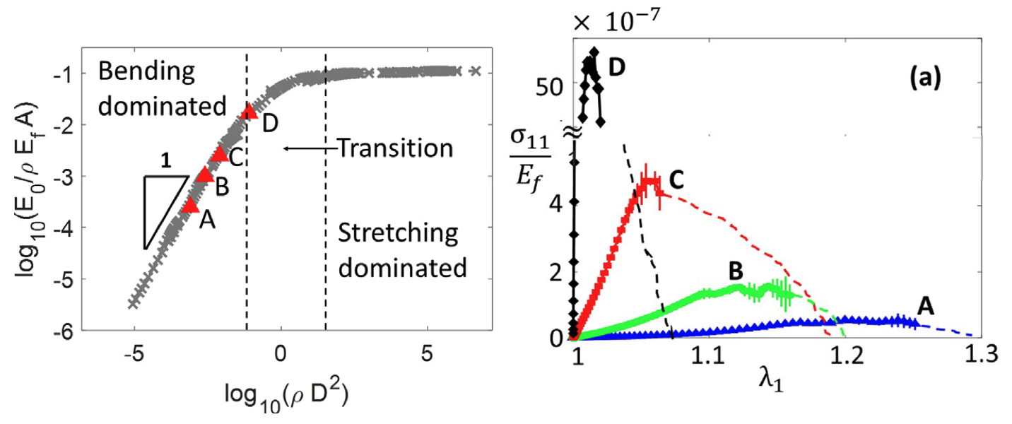
Figure 4 shows numerical results defining the dependence of the network stiffness, E0, on structural parameters.

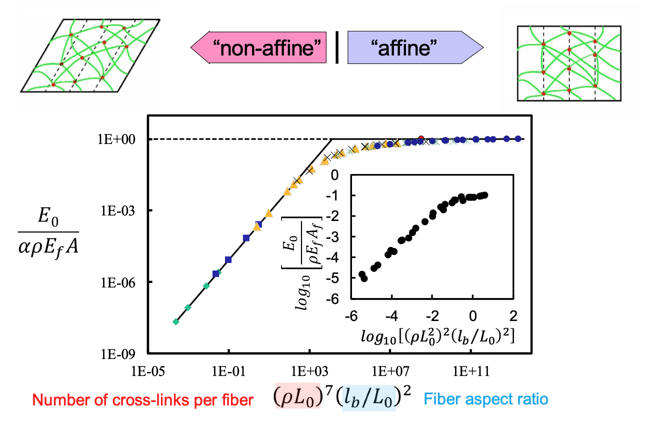
Two regimes are observed: for large values of \(\rho\) and for \(E_{f}l\) much larger than \(E_{f}l\) (large \(l_b\)), the network modulus is propositional to \(\rho\) and \(E_{f}A\). In this regime (right end of the curve in Fig. 4) the strain energy is stored primarily in the axial deformation mode of fibers. For small densities and/or fibers soft in bending, the network modulus is proportional to \(\rho^x\) and \(E_{f}l\) and the strain energy is stored in the bending deformation mode of fibers. Exponent x takes values between 2 (for Voronoi 3D networks) and 8 (for 2D Mikado architecture). Large values of x indicate large sensitivity of network behavior to the density.

• R.C. Picu, “Mechanics of random fiber netwroks – a review,” (invited review article) Soft Matter, Vol. 7, p. 67686785, 2011.
• A.S. Shahsavari, R.C. Picu, “Elasticity of sparsely cross-linked random fiber networks,” Phil. Mag. Lett., Vol. 93, p. 356-361, 2013.
• A.S Shahsavari, R.C. Picu, “Model selection for athermal cross-linked fiber networks,” Phys. Rev. E, Vol. 86, p. 011923(1-4), 2012.

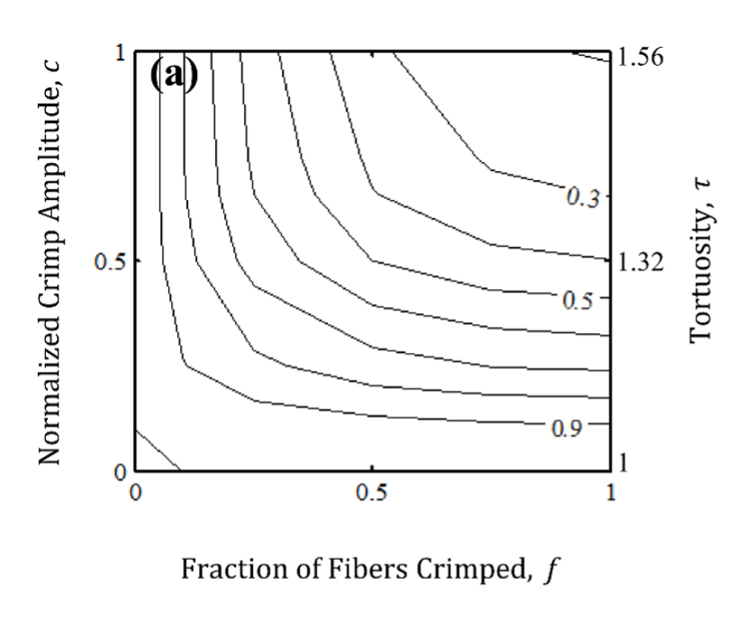
In many cases, fibers are not straight between crosslinks. The stiffness of networks with crimped fibers is much smaller than that of networks of same architecture, but with straight fibers - see Figure 5. The two parameters of the map are the amplitude of crimp (fibers have sinusoidal shape of amplitude cL, where L is the distance between the end nodes) and the fraction of the fibers of the network which are crimped, f.

• E. Ban, V. Barocas, M. Shephard, R.C. Picu, “Effect of fiber crimp on the elasticity of random fiber networks with and without embedding matrices,” J. Appl. Mech., 83, 041008, 2016.

Effect of a matrix embedding

Many networks are embedded in a matrix. Connective tissues are collagen networks embedded in a viscoelastic fluid, while some man-made networks are embedded in elastic continua. As seen above, networks behave in ways different from continua; for example they deform non-affinely, exhibit strain stiffening at larger strains, and have large Poisson ratios. One can ask to what extent the network signature on the overall behavior of such composites is still visible as the embedding material modulus increases. It can be shown that even a very soft elastic matrix eliminates the network behavior to a large extent, i.e. renders the overall modulus largely insensitive to parameters c and f (Fig. 5). The matrix confines the bending mode of fibers and restricts the Poisson contraction to the Poisson ratio of the matrix. A network embedded in a viscoelastic fluid exhibits time-dependent behavior which is described by Poroelasticity. When loaded with high strain rates, the matrix response is solid-like. At low strain rates, the fluid may flow across and in and out of the network (drainage). This process modulates the response of the network.

Damage accumulation and the strength of network materials

Networks usually fail because the rupture of crosslinks. In some other cases – primarily if the network is embedded in a solid matrix – failure implies the rupture of fibers. The failure process can be gradual or catastrophic. A gradual process implies that crosslinks fail in an uncorrelated manner until the fraction of lost crosslinks becomes large enough to destabilize the network. If crosslink rupture is correlated, clusters of crosslinks will rupture at the once which produces a crack-like void. Such defect becomes a crack once large enough.

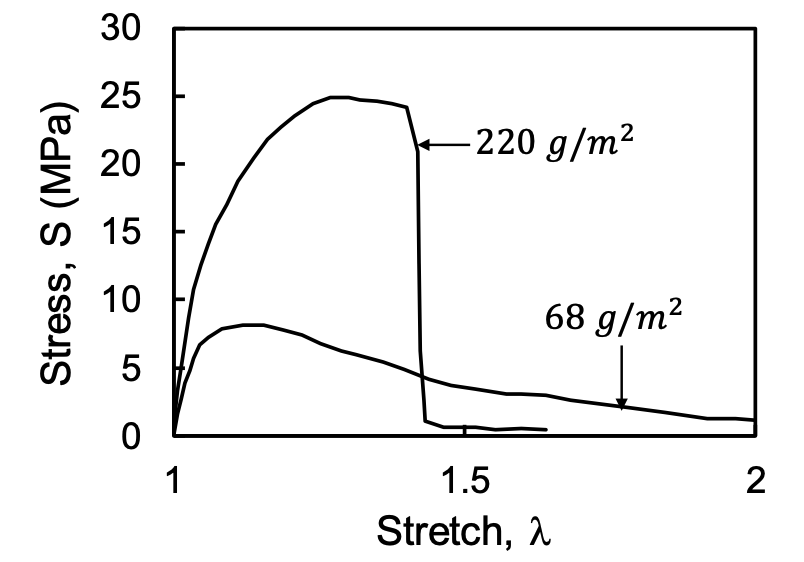
Figure 6 shows typical stress-strain curves for two nonwovens. Densely crosslinked nonwovens reach the maximum stress and fail abruptly; these are brittle materials. Sparsely crosslinked or low density network fail gradually and exhibit a long tail of the stress-strain curve beyond the peak.

This experimental observation is supported by simulations. Figure 7 shows the rupture of 4 types of networks corresponding to different positions on the master curve of Fig. 4. All these networks are non-affine and very soft. We see that network D, which is closer to the affine range, is not only much stiffer, but also has higher strength and is more brittle than network A, which is deep into the non-affine range.

Numerical models have been used to determine the dependence of the strength, \(S_r\), on the various network parameters listed above. It results that the strength is independent of the fiber crimp and fiber properties. The strength scales linearly with the crosslink density, \(r_b\), and with the crosslink (for fiber) strength, \(f_c\). For a broad range of parameters and network architectures, it results that:

\[S_r \sim \rho_b f_c l_c \sim \frac{f_c}{l_{c}^{2}}\]

where lc is the mean segment length of the network.

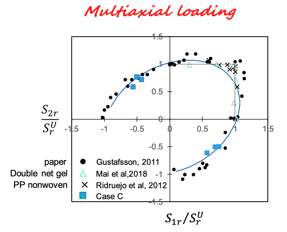
Under multiaxial conditions, the strength of the network can be described by a failure envelope. Figure 8 shows the failure surface for biaxial loading, in the 2D stress space. The two axes are normalized by the strength Sr of each network considered. This normalization makes the failure surfaces of various networks collapse. The plot shows experimental data for paper, a double network gel and a polymer fiber nonwoven.

Warning: The results shown above refer to networks which are not embedded in a solid or viscoelastic fluid. The presence of a matrix alters significantly the failure mode. Likewise, molecular networks in which nonbonded interactions between molecules are important, rupture in ways different from what is presented here. This is because the nonbonded interactions convey a mechanics somewhat similar to that of a network embedded in matrix.

• S. Deogekar, R.C. Picu, On the strength of random fiber networks, J. Mech. Phys. Sol., Vol. 116, pp. 1-16, 2018
• S. Deogekar, M.R. Islam, R.C. Picu, Parameters controlling the strength of stochastic fibrous materials, Int. J. Sol. Struct. Vol. 168, pp. 194-202, 2019.
• S. Deogekar, Z. Yan, R.C. Picu, Random fiber networks with superior properties through network topology control, J. Appl. Mech., Vol. 86, pp. 081010, 2019
• S. Deogekar, R.C. Picu, Strength of stochastic fibrous materials under multiaxial loading, Soft Matter, Vol. 17, pp. 704-714, 2021

Networks with inter-fiber adhesion

Crosslinked networks

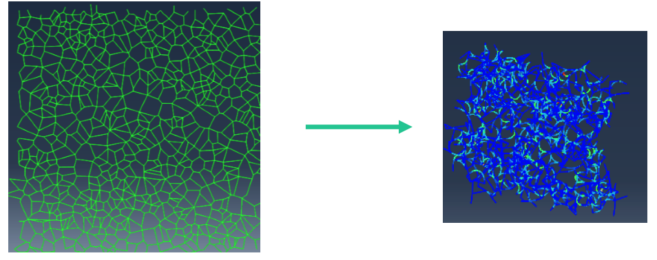
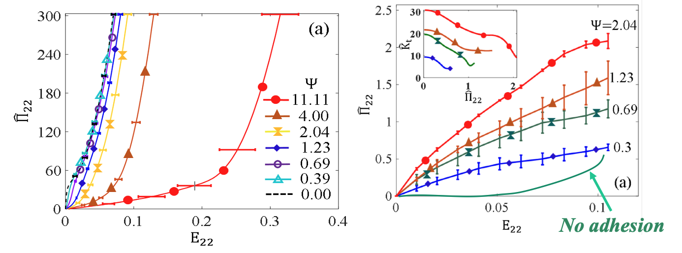
Inter-fiber adhesion modifies drastically the structure and mechanics of networks. Adhesion leads to the collapse of the network and rapid reduction of the free volume, Fig. 9. This process is observed in thermosets whose volume decreases during crosslinking, i.e. as molecular strands are brought closer to each other. The behavior of a collapsed network with inter-fiber adhesion is quite different from that of the same network in which such interactions are not enabled. This is shown in Fig. 10.

• V. Negi, R.C. Picu, Mechanical behavior of cross-linked random fiber networks with inter-fiber adhesion, J. Mech. Phys. Sol., Vol. 122, pp. 418–434, 2019.

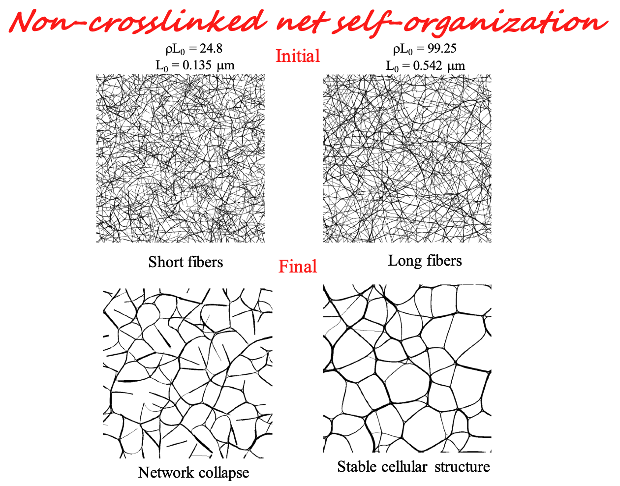
Non-Crosslinked networks

If fibers are not crosslinked, attractive surface interactions lead to bundling and the formation of a network of fiber bundles. Consider the situation in Fig. 11, where quasi-2D networks are first created by depositing straight fibers on a plane. Further, adhesive interactions are turned on and fibers self-organize. If the fiber length is small, the resulting fiber bundles may lose contact and no structure emerges. However, if the fibers are long and the density is high enough, a cellular network of fiber bundles forms. This network has no crosslinks and is stabilized entirely by adhesion.

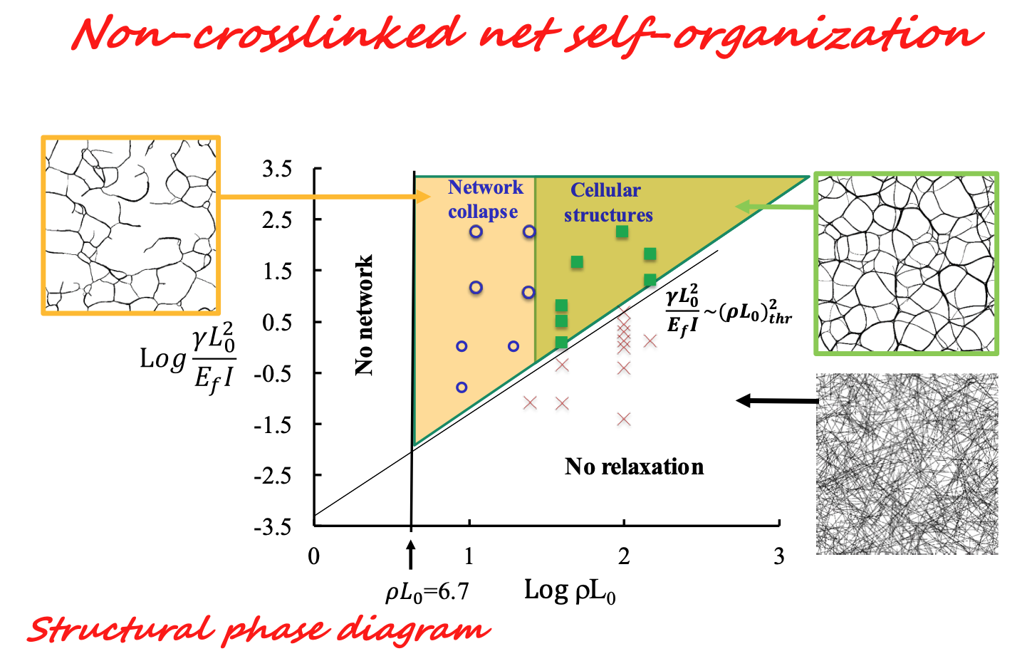
It is possible to define a phase diagram indicating the states of the system for specific network parameters. Figure 12 shows the phase diagram for quasi-2D networks. The horizontal axis represents the non-dimensional group of the horizontal axis of the master plot (Figs. 4 and 7). The vertical axis represents the inverse of the elasto-capilarity length, \(L_{EC}\), i.e. \( (\gamma L_{0}^2)⁄(E_f I)=(L_0⁄L_EC )^2 \), and \(\gamma\) represents the specific surface interaction energy.

• R.C. Picu, A. Sengab, Structural evolution and stability of non-cross-linked fiber networks with inter-fiber adhesion, Soft Matter, Vol. 14, pp. 2254, 2018
• A. Sengab, R.C. Picu, Filamentary structures self-organized due to adhesion, Phys. Rev. E, Vol. 97, pp. 032506, 2018
• V. Negi, R.C. Picu, Mechanical behavior of cellular networks of fiber bundles stabilized by adhesion, Int. J. Sol. Struct., Vol. 190, pp. 119-128, 2020
• V. Negi, R.C. Picu, Mechanical behavior of nonwoven non-crosslinked fibrous mats with adhesion and friction, Soft Matter, Vol. 15, pp. 5951-5964, 2019.
• V. Negi, R.C. Picu, Tensile behavior of non-crosslinked networks of athermal fibers in the presence of entanglements and friction, Soft Matter, Vol. 17, pp. 10186-10197, 2021

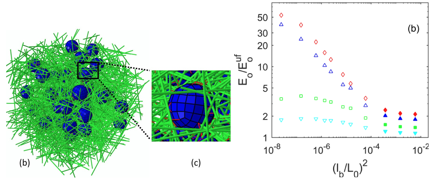
Networks with inclusions

Most network materials contain inclusions of various kinds. In general, inclusions are much stiffer than the network. These systems are composites which differ from the current composites with continuum matrix in that the matrix is a network. The homogenized behavior of such composites has not been explored extensively to date. Figure 13 shows the filled network stiffness, \(E_0\), normalized by the stiffness of the same network without fillers, \( E_0^{uf} \), versus the structural parameter \(l_b\), which represents the bending stiffness of fibers. When the network is in the affine range, i.e. \(l_b\) is large, the stiffening effect of inclusions (multiple volume fractions are shown in Fig. 13) is as expected for a composite with continuum matrix. Specifically, in this range of \(l_b\), the network stiffness increases approximately linearly with the volume fraction. The more interesting regime is that of non-affine networks, with small bending stiffness and small \(l_b\), where the reinforcement effect of fillers is much more pronounced. This enhancement of the stiffening effect increases with decreasing \(l_b\). This effect can be used to engineer soft materials for implants and tissue repair.

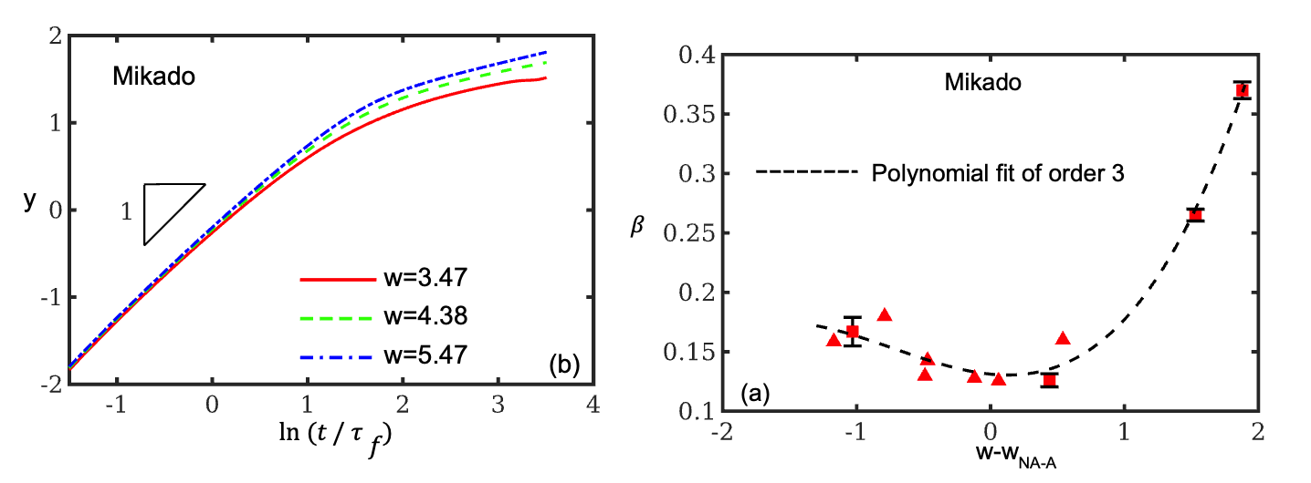
Stress relaxation in networks: Emergence of non-exponential relaxation

Stress relaxation in network materials is mediated by various mechanisms: viscoelasticity of fibers, viscous friction between fibers, contribution of a viscoelastic embedding medium, transport of fluids in and out of the network (poroelasticity). Of these, the first mechanism is least studied. We have shown that if all other mechanisms are turned off and fiber behavior is represented with a Maxwell model, the overall relaxation of the network exhibits two regimes. The first is exponential, with a relaxation time constant similar to that of the fibers. The second regime is described by a stretched exponential function (Kohlrausch relaxation). This indicates that relaxation is fast at the beginning and slows down at later stages. The slowdown is due to network heterogeneity. This phenomenology is similar to relaxation in glass forming polymers in the vicinity of the glass transition temperature. In polymers the control parameter is the temperature and the slowdown is due to heterogeneous dynamics. In stochastic networks of non-evolving architecture, the slowdown is due to the structural heterogeneity of the network and the control parameter is the structural parameter on the horizontal axis of the master plot of Fig. 4.

• N. Amjad, R.C. Picu, Stress relaxation in network materials: the contribution of the network, Soft Matter, in press, 2021.

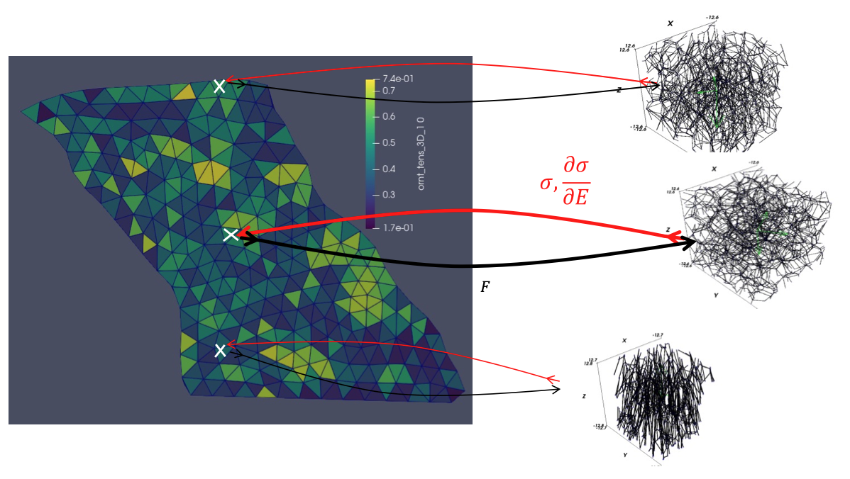
Multiscale models of network materials

Modeling is of great help when trying to understand the mechanics of network materials. However, in most cases, the required models are too large to be tractable with current computational capabilities. This drives the development of multiscale models which may, at once, represent large problem domains and account for the details of the network architecture and mechanics. Figure 15 shows the conceptual schematic of a two-scale method developed by our group, in which the problem domain is represented using finite elements and the constitutive response of each element is dictated by a sub-scale network model. The macroscale continuum provides displacement boundary conditions to the microscale network models, which return to the macroscale the stress in the respective element. The solution requires iterations on both the macro and microscales and is obtained using massively parallel processing.

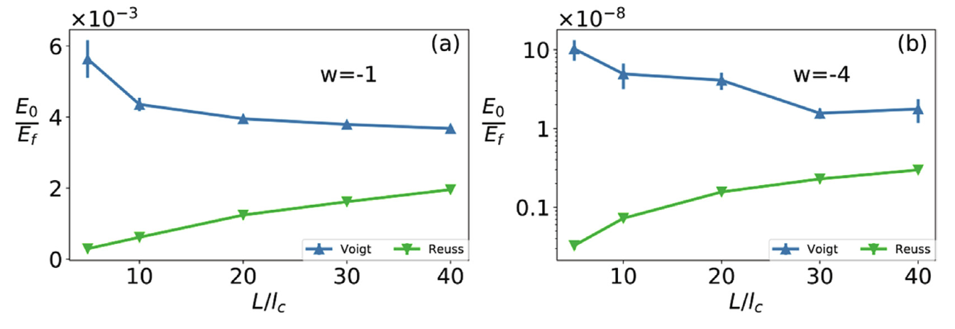
Size effect in networks

Modeling network materials presents difficulties imposed by computational limitations: models in which each filament is represented explicitly (see the subscale models of Fig. 15) are expensive and must be kept sufficiently small to remain manageable. This raises the question of size effects: to what extent the behavior depends on the size of the model used? We studied size effects in networks of various architectures, in 2D and 3D, while focusing on the prediction of stiffness and strength. The main insight resulting from these studies may be summarized as follows: (a) Size effects are pronounced and are due to the intrinsic heterogeneity of the network, (b) Size effects are more pronounced in 3D than in 2D, (c) The size effect of stiffness becomes more pronounced as the network becomes more non-affine (the structural parameter of the horizontal axis in Fig. 4 decreases). (d) Ways to mitigate the size effect exist: we used specially designed flexible boundary conditions which allow computing properties (stiffness) relevant for structures of infinite size using small models. To demonstrate the importance of the size effect, Fig. 16 shows the upper and lower bounds of Voronoi networks vs. the model size, L. The sample size that eliminates the size effect corresponds to L at which the upper and lower bounds merge. This range is not reached even for models as large as 40 times the mean segment length, \(l_c\).

• J. Merson, R.C. Picu, Size effects in random fiber networks controlled by the use of generalized boundary conditions, Int. J. Sol. Struct., Vol. 206, pp. 314-321, 2020.
• S. Shahsavari and C. R. Picu, “Size effect on mechanical behavior of random fiber networks,” International Journal of Solids and Structures, vol. 50, no. 20-21, pp. 3332–3338, Oct. 2013
• S. Deogekar, R.C. Picu, On the strength of random fiber networks, J. Mech. Phys. Sol., Vol. 116, pp. 1-16, 2018

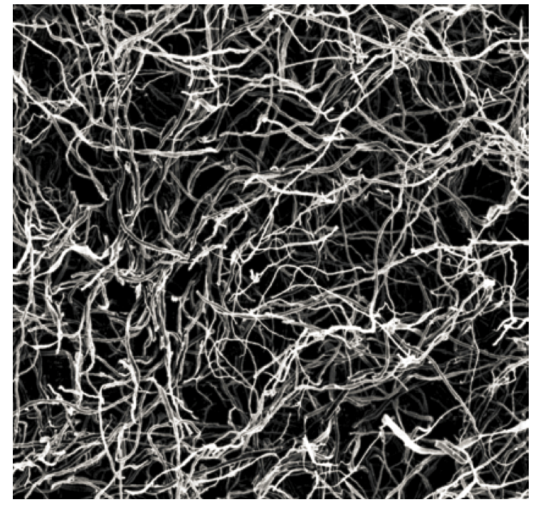
Mycelium

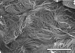
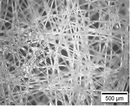
Mycelium is the vegetative part of a fungus. It consists of a colony of tubular filaments called hyphae, which extend in search for food. Such filaments may merge when they meet. The resulting network appears to be branched and is entangled and stochastic. An image of a dried hyphae network is shown in Fig. 17.

Mycelium can be used for various purposes and has become one of the favorite current research topics in network materials. Hyphae network growth can be directed, to some extent, by controlling oxygen and chemical clues. Once it forms, it can be heat treated and dried to remove the organic component, which results in a fibrous material which can be used for packaging and other applications, including food processing. If compacted, it becomes a hard, compact plate which may be used in all applications where engineered wood is desirable.

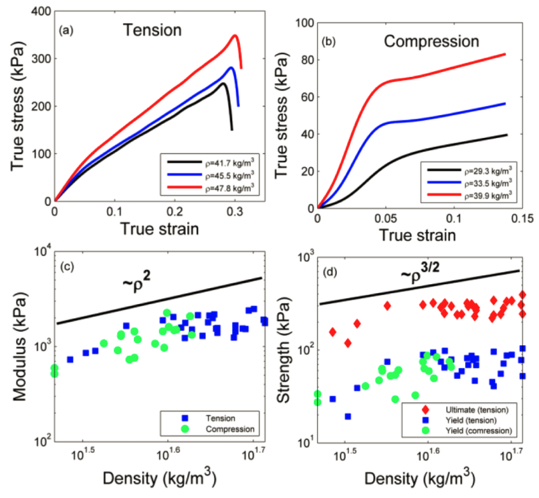
Our lab, in collaboration with Ecovative Inc., performed the first mechanical evaluation of the properties of mycelium, both in network form, and as composite with wood particles. Figure 18 shows stress-strain curves of mycelium (Fig. 17) with different densities, loaded in compression and tension. Further details are available in the articles listed below.

• M.R. Islam, G. Tudryn, R. Bucinell, L. Schadler, R.C. Picu, Morphology and mechanics of fungal mycelium, Scientific Reports, Vol. 7, p. 13070(1-12), 2017
• M.R. Islam, G. Tudryn, R. Bucinell, L. Schadler, R.C. Picu, Mechanical behavior of mycelium-based particulate composites, J. Mater. Sci, Vol. 53, pp. 16371–16382, 2018, DOI 10.1007/s10853-018-2797-z
• M.R. Islam, G. Tudryn, R. Bucinell, L. Schadler, R.C. Picu, Stochastic continuum model for mycelium-based bio-foam, Materials&Design, Vol. 160, pp. 549–556, 2018.