


Density contours at different times for the Rayleigh Taylor Instability
This simulation was performed on a 4 processor intel machine using a non conforming adaptive grid method and our Discontinuous Galerkin code. An animation of both density and mesh evolutions is available here . This next animation shows the evolution of the fluid density for the 1-mode Rayleigh-Taylor with 2 different refinements.
3D Rayleigh Taylor. We have also computed 3D Rayleigh Taylor instabilities on large scale computers like on lemieux or Blue Horizon .
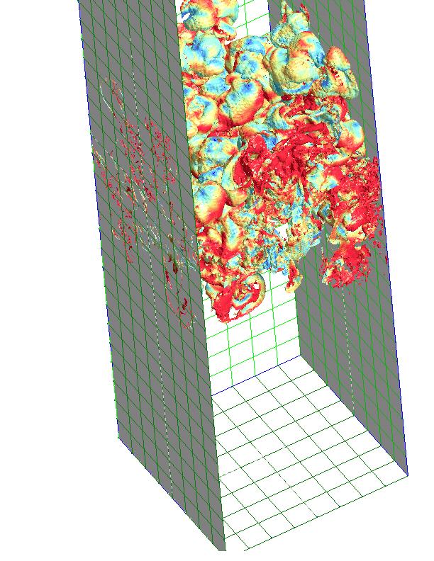
Isosurface of density for a 1-mode and 10-modes 3D Rayleigh Taylor Instability
2D Vortex Sheets. We consider a square domain of size 1 X 1 centered at x=0 and y=0. The problem is initially divided into four quadrants. Quadrant 1 is the upper right, 2 the upper left, 3 the lower left and 4 the lower right. All boundary conditions are transmitting (we copy the interior data perpendicular to the boundary). We initialize each quadrant with the following values for u {density,x velocity, y velocity, pressure}. quantities :
Quadrant 3 : u = {1.0,-0.75, 0.5,1.0} Quadrant 4 : u = {3.0,-0.75,-0.5,1.0}
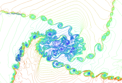
Density contours for the vortex sheet
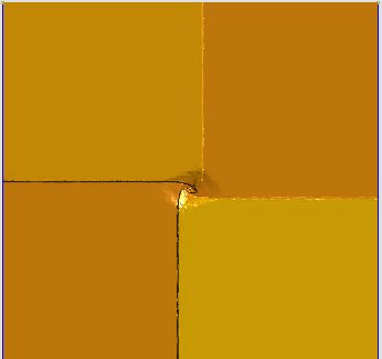
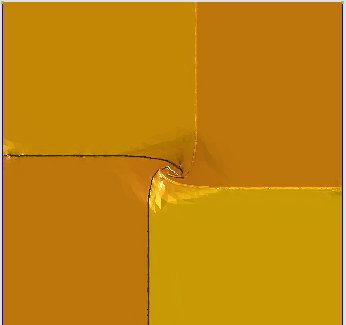

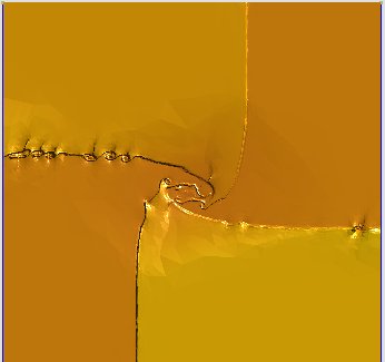
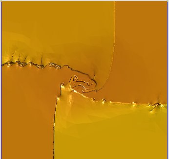
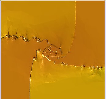
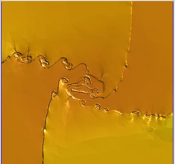
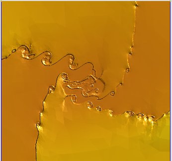
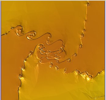
Four Contacts, anisotropic refinement